

Sys 5 Traditional Math: Graphing Pairs of Inequalities
Eighth Grade Algebra

In the previous chapter on graphing, students learned to graph inequalities. Since that time, students have graphed inequalities as part of Warm-Ups, or on a quiz or test to ensure that they maintain that knowledge.
In this lesson, the concept is extended to the graphing of pairs of inequalities. The resulting graphs show the intersection, or common points, of the half-planes represented by the inequalities. The important point is that the intersection contains all and only those points that satisfy both inequalities.
This concept forms the basis for what is called linear programming, a technique used to find the best solution to a problem that may have multiple solutions. It is used in industry to find, say, the maximum production for the least cost. Students usually show an interest in why this is used.
Some students will still find it confusing as to which side of the line gets shaded to represent a particular inequality, so some review may need to be built in to the lesson.


Problem 1 is a review of addition of fractions. Problem 2 is a cost problem in which the total cost is given. Problems 3 and 4 require students to write the inequalities in algebraic form. These problems will be used to introduce the day’s lesson.
Graphing Inequalities. I write on the board:
“I want you to graph this inequality.” I may have to remind them to solve for y first, but they generally remember how to graph inequalities from the lesson given a few lessons back. Seeing that they do this correctly, I then ask them to graph another inequality on the same set of axes.

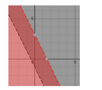
“OK, you’ve all done the first step in graphing pairs of inequalities which is to first draw each line. Now I want you to shade the first one: x + y ≤ 20.” The shaded graph looks like this:

“Now shade the area representing the inequality for the second equation. What side of the line will you shade? Use a different color or a criss-cross pattern.” There will be some messy drawings, but generally, the ones done correctly will resemble the following:

“All the points in this region satisfy both inequalities. Now since we’re dealing with pounds of apples, having negative amounts doesn’t make sense. So we confine the graph to the first quadrant so that both values are positive. All the points in the shaded area satisfy both inequalities.”
I have the students name some points in the shaded area. The point (8,8) is in the shaded area.
“Going back to our original inequalities—before we put them in y=mx+b form. Look at the first one and plug in (8,8) and see if it satisfies the inequality.” Students do this on mini-whiteboards.

“That works; now let’s try the cost inequality.”

“What this is saying is that if you have 8 apples and 8 oranges, you will have less than 20, and selling them at the prices of $8 and $4 per pound or apples and oranges respectively, you will make more than $20. Find some other points.”
Students do so, and as they pick them, I have them tell me what they represent as I just did.
“Now pick some points outside the shaded area.” One such point might be (8, 12). Plugging it in to the original equations, we obtain:

Students may say “But it satisfies that second inequality.” And they would be right. But it doesn’t satisfy the first. “We want to find combinations that satisfy both, and only the points within the shaded area will do that.
Examples. I have them graph more in their notebooks as I go around and check on progress and provide help as necessary. In general, students do well with these.

I give two or more examples to make sure they have the hang of it. Some students still may have a difficult time identifying which side of the graph must be shaded, so I use the same technique in which they look at the y values increasing or decreasing from a particular point on a line. This helps determine which side represents y values greater than or less than the point on the line.
I also include an example similar to the Warm-Ups in which they must translate words into inequalities as indicated in Problem 4.
4. Mary can spend no more than $21 on fruit. Blueberries cost $4/lb and strawberries cost $3/lb. She needs at least 3 pounds of the two fruits to make muffins. Write the inequalities and graph.

Students will need to eyeball the y-intercept for the first equation, but I assure them that the graph does not need to be accurate—we just need a general idea.
Graphing Systems with No Solutions. Students learned in the unit on graphing that lines with equal slopes are parallel. They also learned that a system of two parallel lines has no solution. I remind them of this and have them graph the following lines:

They will get two parallel lines:

“Now I’m going to state these as inequalities and I want you to shade in the graph.”

They will get this result:

“Is there a solution for these inequalities?”
The general answer is “No” which is correct. “There is no common area in the graph, so we say there is no solution. But now, what if we had these inequalities? Sketch this on a different set of axes.”
“Now we have a solution in the narrow pipeline. All the points in the common area are solutions for these two inequalities.”
Homework. The homework consists of graphing pairs of linear inequalities, some of which are word problems in which they have to write the inequalities and graph them, as was done at the beginning of the lesson. Other problems require graphing the inequalities, as well as identifying the systems of inequalities from a graph.